A. Required R packages

We will use several R packages. Firstly, tidyverse family functions will be used to create a statistical summary, which is a data table of class data.frame. The pipe operator %>% will be used to join several functions into one sequence. Secondly, package flextable will be used to convert the table to the format that can be saved as a Word table. Finally, package officer will be used to save the table.

# Download and install packages from CRAN 
install.packages(c("tidyverse", "flextable", "officer"))

# Load necessary packages
library(tidyverse)
library(flextable)
library(officer)

B. Settings: locale

A locale can be defined as a language and location dependent set of program parameters and properties. If we would like use, e.g., Lithuanian symbols, we would set the Lithuanian locale.

# Set locale on Windows
Sys.setlocale(locale = "Lithuanian")

# Set locale on Mac OS and most of Linux distributions
Sys.setlocale(locale = "lt_LT.UTF-8")

# Set locale on some of Linux distributions
Sys.setlocale(locale = "lt_LT.utf8")

To check your current locale, you can write Sys.getlocale() and use the result as an exaple to choose correct syntax for setting the locale. More on locales in R documentation.

In this post, we do not need to change the locale.

C. Load your data

It’s time to import data. In this post, we will use dataset “PlantGrowth” from package datasets.

# Import data
data("PlantGrowth", package = "datasets")

Let’s look at data. A few top rows:

# Top rows
head(PlantGrowth)
##   weight group
## 1   4.17  ctrl
## 2   5.58  ctrl
## 3   5.18  ctrl
## 4   6.11  ctrl
## 5   4.50  ctrl
## 6   4.61  ctrl

The structure of the dataset:

# The structure of the dataset
glimpse(PlantGrowth)
## Observations: 30
## Variables: 2
## $ weight <dbl> 4.17, 5.58, 5.18, 6.11, 4.50, 4.61, 5.17, 4.53, 5.33, 5...
## $ group  <fct> ctrl, ctrl, ctrl, ctrl, ctrl, ctrl, ctrl, ctrl, ctrl, c...

Here “Observations” represent the number of rows and “Variables” – the number of columns. Column/Variable names in each new row and are preceded by $. These names are followed by abbreviated data type (<dbl>, double – real numbers, <fct>, factor – categorical variables) and several first values.

Write help("PlantGrowth", package = "datasets") to read full documentation of the dataset.

D. Make a statistical summary

Now we are going to create a statistical summary in the form of R data.frame: to calculate the mean and standard deviation of weight by group and a size of each group. The functions group_by() and summarize() from package dplyr are handy for this purpose. Next, we will rename() from group to Group name to make the summary look more beautiful.

# Create a summary
my_summary_as_df  <- 
    PlantGrowth %>% 
    group_by(group) %>%
    summarize("Group size"  = n(),
              "Mean weight" = mean(weight),
              "Standard deviation" = sd(weight)) %>% 
    rename("Group name" = group)

Let’s print the summary.

my_summary_as_df 
## # A tibble: 3 x 4
##   `Group name` `Group size` `Mean weight` `Standard deviation`
##   <fct>               <int>         <dbl>                <dbl>
## 1 ctrl                   10          5.03                0.583
## 2 trt1                   10          4.66                0.794
## 3 trt2                   10          5.53                0.443

If you see this kind of output for the first time, it may look very technical. Yet, you should notice, that the size of group ctrl is 10 and the mean weight is approximately 5.03. You should also notice that the class of this table is data.frame (the last word in the next output):

# Object's class
class(my_summary_as_df )
## [1] "tbl_df"     "tbl"        "data.frame"

In the subsequent chapter, you can use any data frame. This one was created for demonstration purposes only. However, if your summary is not a data.frame, the following method is not applicable.

E. Make the table to be exportable to Word

Before exporting the table to Word, the table should be converted into an appropriate form that can be exported. For this purpose, the function regulartable() from package flextable are used. Optionally, the function autofit() can be used to optimize the size of the table (the heights of the rows and the widths of the columns).

my_summary_to_save <- my_summary_as_df %>% regulartable() %>% autofit()

Let’s look at the table:

my_summary_to_save 

F. Round the numbers

By default, integers are not rounded up, and real numbers are rounded to 3 decimal places. If such rounding is not appropriate, we can specify it for each type of numeric variables separately using the function set_formatter_type() {.r}. Usually, the rounding should be specified for real numbers only and can be defined by the following line: '% .6f' {.r}. Here % indicates the beginning of the format (fmt) description, f shows a fixed format, and a number after a point defines how many decimal places the number should be rounded to (in this example, 6). The lines of code that control the rounding of real (double) numbers:

# Set default rounding for real numbers
my_summary_to_save_2  <- 
    my_summary_to_save  %>% 
    set_formatter_type(fmt_double = "%.6f")  

my_summary_to_save_2 

We can also set the rounding for each selected variable separately using function set_formatter(), quoted variable name and the following syntax:

# Set rounding for each variable separately
my_summary_to_save_3  <- 
    my_summary_to_save_2 %>% 
    set_formatter( 
        "Mean weight"        = function(x) sprintf("%.2f", x),
        "Standard deviation" = function(x) sprintf("%.1f", x)
    )

In format description, we should write the number of decimal places we are interested in.

my_summary_to_save_3

Of course, rounding to 6 decimal places as well as different rounding for mean and standard deviation are irrelevant. So we will not use these cases of rounding in the following chapters. They served as examples only.

G. Export to Word

Next, we use read_docx() (from the package officer) to create a new Word document, body_add_flextable() to add our table to this document, and print() to save the Word document (I’m surprised that print() is used to save a document, but this was the choice of the package authors). The parameter target allows specifying the desired name of the Word document in which the file extension (the last letters after the dot) must be “.docx”, as in this example:

word_document_name <-
    read_docx() %>%
    body_add_flextable(my_summary_to_save) %>%
    print(target = "document_with_summary.docx")

After saving the Word document, the sequence of functions outputs the document name. You can verify this by printing variable word_document_name.

Note If a warning is issued that the document can not be saved, check that there is no any other Word document with the same name (in this case “document_with_summary.docx”) opened.

Warning! If your current working directory (the folder R tries to write the document in) already contains a document with the same name, then running the code will overwrite it without any alert. So when you open the Word document and edit the table, I recommend changing its name.

H. Open the Word document

When the table is exported to Word, you can open the document and see the result by using the following line of code:

# Open the document
browseURL(word_document_name)

The result in the „Word“ document is going to look like this one:

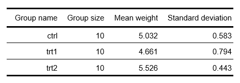
Figure 1: The table in a „Word“ document.

The full script

Finally, I present the full script: copy it and suit your needs by replacing or deleting (un)necessary lines.

# A. Load packages
library(tidyverse)
library(flextable)
library(officer)

# B. Set locale (if needed)
# Sys.setlocale(locale = "Lithuanian")

# C. Import data
data("PlantGrowth", package = "datasets")

# D. Make a summary (i.e., a data frame)
my_summary_as_df <-
    PlantGrowth %>%
    group_by(group) %>%
    summarize("Group size" = n(),
              "Mean weight" = mean(weight),
              "Standard deviation" = sd(weight)) %>% 
    rename("Group name" = group)

# E. Prepare data.frame for saving
my_summary_to_save <-
    my_summary_as_df %>%
    regulartable()   %>%
    autofit()

# F. Round the numbers (if needed)
my_summary_to_save <- 
    my_summary_to_save %>% 
    
    # Default rounding for real numbers
    set_formatter_type(fmt_double = "%.3f") %>% 
    
    # Rounding for each variable separately
    set_formatter( 
        "Mean weight"        = function(x) sprintf("%.3f", x),
        "Standard deviation" = function(x) sprintf("%.3f", x)
    )

# G. Save as a Word table
word_document_name <-
    read_docx() %>%
    body_add_flextable(my_summary_to_save) %>%
    print(target = "document_with_summary.docx")

# H. Open the Word document 
browseURL(word_document_name)

Good luck!